Data migration
The dataset is stored in a CSV file format and is hosted on Kaggle. To facilitate data migration and analysis, we will use Google BigQuery, a serverless, highly scalable, and cost-effective cloud data warehouse provided by Google Cloud Platform. BigQuery allows us to run SQL-like queries on large datasets and perform complex analytics tasks with ease.
To access the dataset in BigQuery, we first need to upload the CSV file to Google Cloud Storage (GCS). From there, we can create a new dataset in BigQuery and import the data from GCS into a new table. Once the data is loaded into BigQuery, we can start querying the dataset using SQL commands and perform various data analysis tasks.
The following steps outline the process of migrating the dataset to BigQuery:
- Upload the CSV file to Google Cloud Storage (GCS).
- Create a new dataset in BigQuery.
- Import the data from GCS into a new table in BigQuery.
- Query the dataset using SQL commands in BigQuery.
To see the detailed steps for migrating the dataset to BigQuery, click here.
Model preparation
Before building a predictive model for diabetes risk assessment, we need to prepare the dataset for training and testing. This involves several steps, including data preprocessing, feature engineering, and splitting the data into training and testing sets.
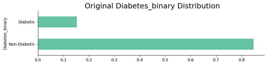
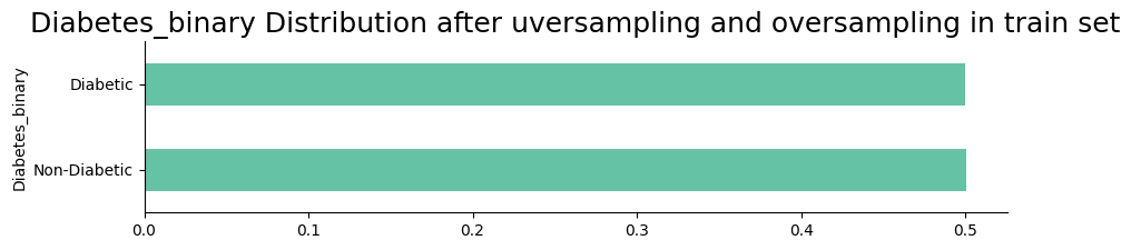
The dataset is imbalanced, requiring the application of techniques such as NearMiss and SMOTE (Synthetic Minority Oversampling Technique). NearMiss helps by under-sampling the majority class, focusing on samples close to the decision boundary, while SMOTE generates synthetic samples for the minority class to create a more balanced dataset. These preprocessing steps are crucial for improving the model's ability to generalize and perform effectively across all classes.
Once the data is preprocessed, we will split it into training and testing sets using a stratified approach to maintain the class balance in the target variable. This will allow us to train the model on a subset of the data and evaluate its performance on unseen data.
The following steps outline the process of preparing the dataset for model training:
- Preprocess the data by encoding categorical variables and scaling continuous variables.
- Split the data into training and testing sets using a stratified approach.
- Train the model on the training set and evaluate its performance on the testing set.
Data distribution after processing
The following visualizations show the distribution of the target variable after applying data preprocessing techniques such as NearMiss and SMOTE. The plots illustrate the balance achieved in the target variable, which is essential for building an effective predictive model.
Results from the models
After training the model on the preprocessed dataset, we evaluate its performance using various metrics such as accuracy, precision, recall, and ROC curve. These metrics provide insights into how well the model is performing in predicting diabetes risk and help us assess its effectiveness in differentiating between diabetic and non-diabetic cases.
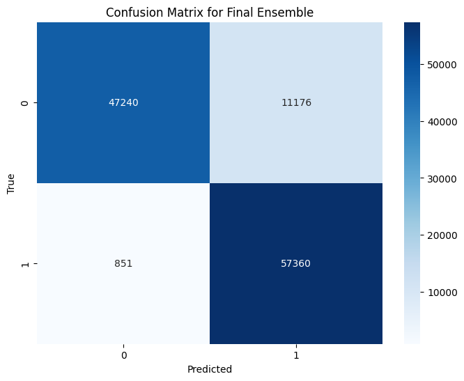
Confusion matrix
The confusion matrix is a useful tool for visualizing the performance of a classification model. It shows the true positive, true negative, false positive, and false negative values, allowing us to evaluate the model's accuracy and identify any misclassifications.
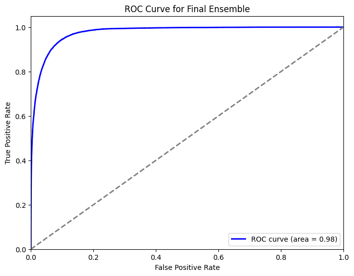
ROC curve
The ROC curve is another important metric for evaluating the performance of a classification model. It plots the true positive rate against the false positive rate at various threshold values, providing insights into the model's ability to discriminate between classes.